Note

This tutorial was generated from a Jupyter notebook that can be downloaded here. If you’d like to reproduce the results in the notebook, or make changes to the code, we recommend downloading this notebook and running it with Jupyter as certain cells (mostly those that change plot styles) are excluded from the tutorials.

Quickstart

In this tutorial, we explain how to quickly use LEGWORK to calculate the detectability of a collection of sources.

Let’s start by importing the source and visualisation modules of LEGWORK and some other common packages.

import legwork.source as source
import legwork.visualisation as vis

import numpy as np
import astropy.units as u
import matplotlib.pyplot as plt

Next let’s create a random collection of possible LISA sources in order to assess their detectability.

# create a random collection of sources
n_values = 1500
m_1 = np.random.uniform(0, 10, n_values) * u.Msun
m_2 = np.random.uniform(0, 10, n_values) * u.Msun
dist = np.random.normal(8, 1.5, n_values) * u.kpc
f_orb = 10**(-5 * np.random.power(3, n_values)) * u.Hz
ecc = 1 - np.random.power(5, n_values)

We can instantiate a Source class using these random sources in order to analyse the population. There are also a series of optional parameters which we don’t cover here but if you are interested in the purpose of these then check out the Using the Source Class tutorial.

sources = source.Source(m_1=m_1, m_2=m_2, ecc=ecc, dist=dist, f_orb=f_orb)

This Source class has many methods for calculating strains, visualising populations and more. You can learn more about these in the Using the Source Class tutorial. For now, we shall focus only on the calculation of the signal-to-noise ratio.

Therefore, let’s calculate the SNR for these sources. We set verbose=True to give an impression of what sort of sources we have created. This function will split the sources based on whether they are stationary/evolving and circular/eccentric and use one of 4 SNR functions for each subpopulation.

snr = sources.get_snr(verbose=True)

Calculating SNR for 1500 sources
        0 sources have already merged
        1396 sources are stationary
                403 sources are stationary and circular
                993 sources are stationary and eccentric
        104 sources are evolving
                24 sources are evolving and circular
                80 sources are evolving and eccentric

These SNR values are now stored in sources.snr and we can mask those that don’t meet some detectable threshold.

detectable_threshold = 7
detectable_sources = sources.snr > 7
print("{} of the {} sources are detectable".format(len(sources.snr[detectable_sources]), n_values))

580 of the 1500 sources are detectable

And just like that we know the number of detectable sources! It could be interesting to see how the SNR varies with orbital frequency so let’s use the legwork.source.Source.plot_source_variables() to create a 2D density distribution of these variables.

fig, ax = sources.plot_source_variables(xstr="f_orb", ystr="snr", disttype="kde", log_scale=(True, True),
                                        fill=True, xlim=(2e-6, 2e-1), which_sources=sources.snr > 0)

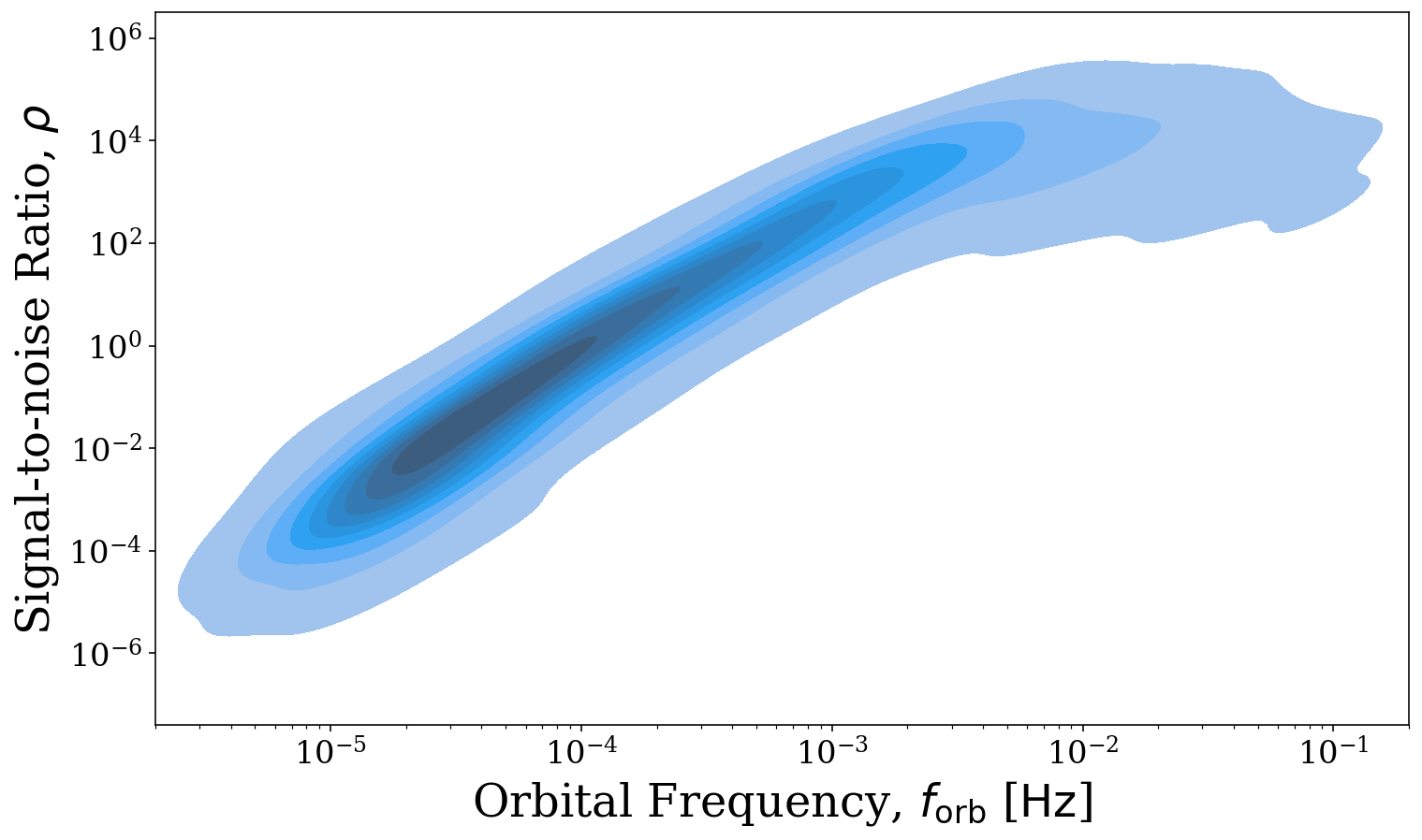
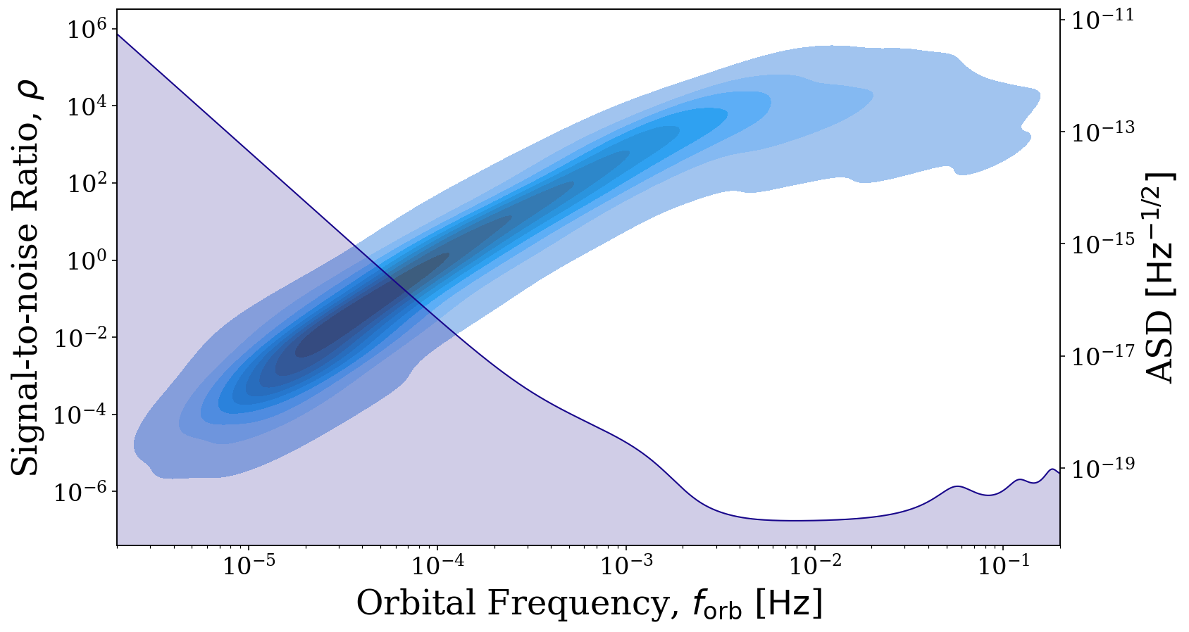
The reason for this shape may not be immediately obvious. However, if we also use the visualisation module to overlay the LISA sensitivity curve, it becomes clear that the SNRs increase in step with the decrease in the noise and flatten out as the sensitivity curve does as we would expect. To learn more about the visualisation options that LEGWORK offers, check out the Visualisation tutorial.

# create the same plot but set `show=False`
fig, ax = sources.plot_source_variables(xstr="f_orb", ystr="snr", disttype="kde", log_scale=(True, True),
                                        fill=True, show=False, which_sources=sources.snr > 0)

# duplicate the x axis and plot the LISA sensitivity curve
right_ax = ax.twinx()
frequency_range = np.logspace(np.log10(2e-6), np.log10(2e-1), 1000) * u.Hz
vis.plot_sensitivity_curve(frequency_range=frequency_range, fig=fig, ax=right_ax)

plt.show()

That’s it for this quickstart into using LEGWORK. For more details on using LEGWORK to calculate strains, evolve binaries and visualise their distributions check out the other tutorials and demos in these docs! You can also read more about the scope and limitations of LEGWORK on this page.