Note
This tutorial was generated from a Jupyter notebook that can be downloaded here. If you’d like to reproduce the results in the notebook, or make changes to the code, we recommend downloading this notebook and running it with Jupyter as certain cells (mostly those that change plot styles) are excluded from the tutorials.
Demo - LISA Horizon Distance
This demo shows how to use LEGWORK to compute the horizon distance for a collection of sources.
[2]:
import legwork as lw
import numpy as np
import astropy.units as u
import matplotlib.pyplot as plt
[3]:
%config InlineBackend.figure_format = 'retina'

plt.rc('font', family='serif')
plt.rcParams['text.usetex'] = False
fs = 24

# update various fontsizes to match
params = {'figure.figsize': (12, 8),
          'legend.fontsize': fs,
          'axes.labelsize': fs,
          'xtick.labelsize': 0.9 * fs,
          'ytick.labelsize': 0.9 * fs,
          'axes.linewidth': 1.1,
          'xtick.major.size': 7,
          'xtick.minor.size': 4,
          'ytick.major.size': 7,
          'ytick.minor.size': 4}
plt.rcParams.update(params)
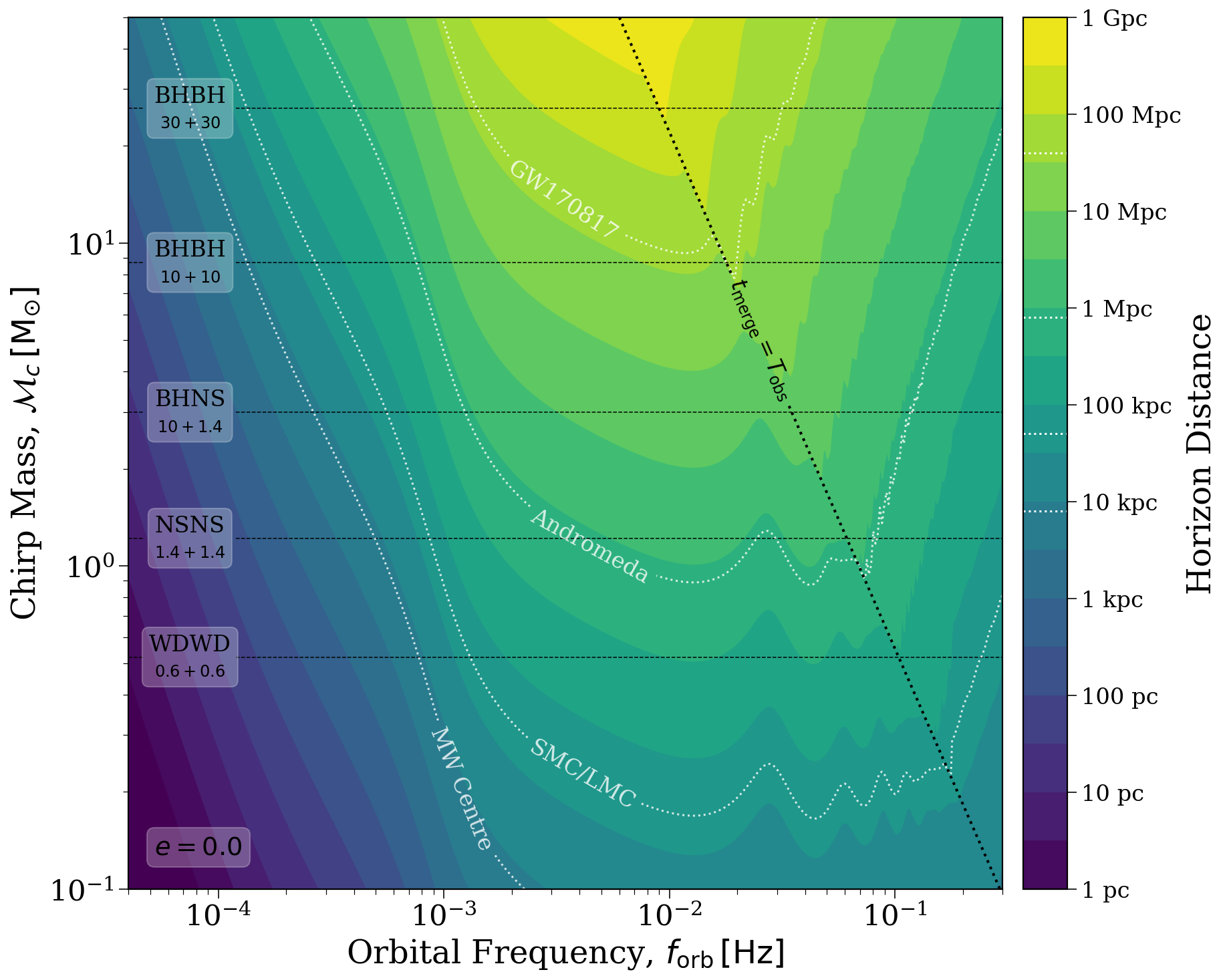
Horizon distance of circular binaries
The horizon distance for a source is the maximum distance at which the SNR of a source is still above some detectable threshold. The horizon distance can be computed from the SNR as follows since it is inversely proportional to the distance.
\begin{equation} D_{\rm hor} = \frac{\rho(D)}{\rho_{\rm detect}} \cdot D, \label{eq:snr_to_hor_dist} \end{equation}
Where \(\rho(D)\) is the SNR at some distance \(D\) and \(\rho_{\rm detect}\) is the SNR above which we consider a source detectable.
Let’s start doing this by creating a grid of chirp masses and orbital frequencies and creating a Source class from them.
[4]:
# create a list of masses and frequencies
m_c_grid = np.logspace(-1, np.log10(50), 500) * u.Msun
f_orb_grid = np.logspace(np.log10(4e-5), np.log10(3e-1), 400) * u.Hz

# turn the two lists into grids
MC, FORB = np.meshgrid(m_c_grid, f_orb_grid)

# flatten grids
m_c, f_orb = MC.flatten(), FORB.flatten()

# convert chirp mass to individual masses for source class
q = 1.0
m_1 = m_c / q**(3/5) * (1 + q)**(1/5)
m_2 = m_1 * q

# use a fixed distance and circular binaries
dist = np.repeat(1, len(m_c)) * u.kpc
ecc = np.zeros(len(m_c))

# create the source class
sources = lw.source.Source(m_1=m_1, m_2=m_2, dist=dist, f_orb=f_orb, ecc=ecc, gw_lum_tol=1e-3)
Next, we can use LEGWORK to compute their merger times and SNRs for the contours.
[5]:
# calculate merger times and then SNR
sources.get_merger_time()
sources.get_snr(verbose=True)
Calculating SNR for 200000 sources
        0 sources have already merged
        125169 sources are stationary
                125169 sources are stationary and circular
        74831 sources are evolving
                74831 sources are evolving and circular
[5]:
array([5.37039831e-04, 5.48303595e-04, 5.59803603e-04, ...,
       1.06420933e+04, 1.07531750e+04, 1.08654183e+04])
We flattened the grid to fit into the Source class but now we can reshape the output to match the original grid.
[6]:
# reshape the output into grids
t_merge_grid = sources.t_merge.reshape(MC.shape)
snr_grid = sources.snr.reshape(MC.shape)
Now we can define a couple of functions for formatting the time, distance and galaxy name contours.
[7]:
def fmt_time(x):
    if x == 4:
        return r"$t_{\rm merge} = T_{\rm obs}$"
    elif x >= 1e9:
        return "{0:1.0f} Gyr".format(x / 1e9)
    elif x >= 1e6:
        return "{0:1.0f} Myr".format(x / 1e6)
    elif x >= 1e3:
        return "{0:1.0f} kyr".format(x / 1e3)
    elif x >= 1:
        return "{0:1.0f} yr".format(x)
    elif x >= 1/12:
        return "{0:1.0f} month".format(x * 12)
    else:
        return "{0:1.0f} week".format(x * 52)

def fmt_dist(x):
    if x >= 1e9:
        return "{0:1.0f} Gpc".format(x / 1e9)
    elif x >= 1e6:
        return "{0:1.0f} Mpc".format(x / 1e6)
    elif x >= 1e3:
        return "{0:1.0f} kpc".format(x / 1e3)
    else:
        return "{0:1.0f} pc".format(x)

def fmt_name(x):
    if x == np.log10(8):
        return "MW Centre"
    elif x == np.log10(50):
        return "SMC/LMC"
    elif x == np.log10(800):
        return "Andromeda"
    elif x == np.log10(40000):
        return "GW170817"
Finally, we put it all together to create a contour plot with all of the information.
[8]:
# create a square figure plus some space for a colourbar
size = 12
cbar_space = 2
fig, ax = plt.subplots(figsize=(size + cbar_space, size))

# set up scales early so contour labels show up nicely
ax.set_xscale("log")
ax.set_yscale("log")

# set axes labels and lims
ax.set_xlabel(r"Orbital Frequency, $f_{\rm orb} \, [\rm Hz]$")
ax.set_ylabel(r"Chirp Mass, $\mathcal{M}_c \, [\rm M_{\odot}]$")
ax.set_xlim(4e-5, 3e-1)

# calculate the horizon distance
snr_threshold = 7
horizon_distance = (snr_grid / snr_threshold * 1 * u.kpc).to(u.kpc)

# set up the contour levels
distance_levels = np.arange(-3, 6 + 0.5, 0.5)
distance_tick_levels = distance_levels[::2]

# plot the contours for horizon distance
distance_cont = ax.contourf(FORB, MC, np.log10(horizon_distance.value), levels=distance_levels)

# hide edges that show up in rendered PDFs
for c in distance_cont.collections:
    c.set_edgecolor("face")

# create a colour with custom formatted labels
cbar = fig.colorbar(distance_cont, ax=ax, pad=0.02, ticks=distance_tick_levels, fraction=cbar_space / (size + cbar_space))
cbar.ax.set_yticklabels([fmt_dist(np.power(10, distance_tick_levels + 3)[i]) for i in range(len(distance_tick_levels))])
cbar.set_label(r"Horizon Distance", fontsize=fs)
cbar.ax.tick_params(axis="both", which="major", labelsize=0.7 * fs)

# annotate the colourbar with some named distances
named_distances = np.log10([8, 50, 800, 40000])
for name in named_distances:
    cbar.ax.axhline(name, color="white", linestyle="dotted")

# plot the same names as contours
named_cont = ax.contour(FORB, MC, np.log10(horizon_distance.value), levels=named_distances,
                        colors="white", alpha=0.8, linestyles="dotted")
ax.clabel(named_cont, named_cont.levels, fmt=fmt_name, use_clabeltext=True, fontsize=0.7*fs,
          manual=[(1.1e-3, 2e-1), (4e-3, 2.2e-1), (4e-3,1e0), (3e-3, 1.2e1)])

# add a line for when the merger time becomes less than the inspiral time
time_cont = ax.contour(FORB, MC, t_merge_grid.to(u.yr).value, levels=[4],
                       colors="black", linewidths=2, linestyles="dotted") #[1/52, 1/12, 4, 1e2, 1e3, 1e4, 1e5, 1e6, 1e7, 1e8, 1e9, 1e10]
ax.clabel(time_cont, time_cont.levels, fmt=fmt_time, fontsize=0.7*fs, use_clabeltext=True, manual=[(2.5e-2, 5e0)])

# plot a series of lines and annotations for average DCO masses
for m_1, m_2, dco in [(0.6, 0.6, "WDWD"), (1.4, 1.4, "NSNS"),
                      (10, 1.4, "BHNS"), (10, 10, "BHBH"), (30, 30, "BHBH")]:
    # find chirp mass
    m_c_val = lw.utils.chirp_mass(m_1, m_2)

    # plot lines before and after bbox
    ax.plot([4e-5, 4.7e-5], [m_c_val, m_c_val],
            color="black", lw=0.75, zorder=1, linestyle="--")
    ax.plot([1.2e-4, 1e0], [m_c_val, m_c_val],
            color="black", lw=0.75, zorder=1, linestyle="--")

    # plot name and bbox, then masses below in smaller font
    ax.annotate(dco + "\n", xy=(7.5e-5, m_c_val), ha="center", va="center", fontsize=0.7*fs,
               bbox=dict(boxstyle="round", fc="white", ec="white", alpha=0.25))
    ax.annotate(r"${{{}}} + {{{}}}$".format(m_1, m_2),
               xy=(7.5e-5, m_c_val * 0.95), ha="center", va="top", fontsize=0.5*fs)

# ensure that everyone knows this only applies for circular sources
ax.annotate(r"$e = 0.0$", xy=(0.03, 0.04), xycoords="axes fraction", fontsize=0.8*fs,
            bbox=dict(boxstyle="round", fc="white", ec="white", alpha=0.25))

ax.set_facecolor(plt.get_cmap("viridis")(0.0))

plt.show()